wf.plot_timeseries(parameters_to_plot=None, qc_flags=None, rolling_window=None, ax=None, average_time=None, secondary_y=None, color=None)

Reference

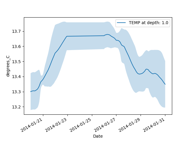
Plot the input parameters with time on X and the parameters on Y. It calculates the standar deviation of a rolling window and plot it.

Parameters

• parameters_to_plot: Parameters of the WaterFrame to plot. If parameters_to_plot is None, all parameters will be ploted. (list of str, str)
• qc_flags: QC flags of the parameters to plot. If qc_flags in None, all QC flags will be used. (list of int)
• rolling_window: Size of the moving window. It is the number of observations used for calculating the statistic.(int)
• ax: It is used to add the plot to an input axes object. (matplotlib.axes object)
• average_time: It calculates an average value of a time interval. You can find all of the resample options here. (str)
• secondary_y: Plot on the secondary y-axis. (bool)
• color: Any matplotlib color. It will be applied to the traces. (str or list of str)

Returns

• ax: Axes of the plot. (matplotlib.AxesSubplot)

Example

To reproduce the example, download the NetCDF file here and save it as example.nc in the same pyhon script folder.

import matplotlib.pyplot as plt
import mooda as md

path_netcdf = 'example.nc'  # Path of the NetCDF file

wf = md.read_nc_emodnet(path_netcdf)

# Plot the sea water temperature
wf.plot_timeseries('TEMP')
plt.show()

Output:

Notes: In this case, “depth: 1.0” means 20 meters of depth. The underwater laboratory OBSEA only measures the seawater temperature at one unique depth, at 20 meters.

Return to mooda.WaterFrame.